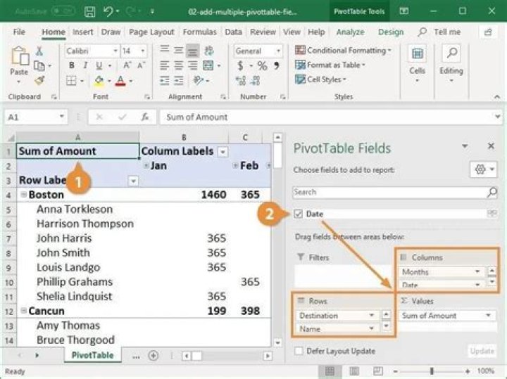
Click any cell in the pivot table layout.The PivotTable Field List pane should appear at the right of the Excel window, when a pivot cell is selected.If the PivotTable Field List pane does not appear click the Analyze tab on the Excel Ribbon, and then click the Field List command.
How can I see the source of a PivotTable?
On the Ribbon, under the PivotTable Tools tab, click the Analyze tab (in Excel 2010, click the Options tab). In the Data group, click the top section of the Change Data Source command. The Change PivotTable Data Source dialog box opens, and you can see the the source table or range in the Table/Range box.
How do I remove grand total from pivot table in Excel?
- Right-click anywhere on your pivot table.
- Select PivotTable Options. …
- Click the Totals & Filters tab.
- Click the Show Grand Totals for Rows check box to deselect it.
- Click the Show Grand Totals for Columns check box to deselect it.
How do I use PivotTable editor?
Edit a pivot table. Click anywhere in a pivot table to open the editor. Add data—Depending on where you want to add data, under Rows, Columns, or Values, click Add. Change row or column names—Double-click a Row or Column name and enter a new name.How do I change the range of a pivot table?
Answer:Select the Options tab from the toolbar at the top of the screen. In the Data group, click on Change Data Source button. When the Change PivotTable Data Source window appears, change the Table/Range value to reflect the new data source for your pivot table. Click on the OK button.
How do I see all pivot tables in a workbook?
1. Open your workbook that you want to list all the pivot tables. 2. Hold down the ALT + F11 keys, and it opens the Microsoft Visual Basic for Applications window.
How do I change data source for multiple pivot tables?
You can change the data source of a PivotTable to a different Excel table or a cell range, or change to a different external data source. Click the PivotTable report. On the Analyze tab, in the Data group, click Change Data Source, and then click Change Data Source.
How do I edit a pivot table in Excel 2016?
In the Data group, click on Change Data Source button and select “Change Data Source” from the popup menu. When the Change PivotTable Data Source window appears, change the Table/Range value to the new data source that you want for your pivot table and then click on the OK button.How do I extract raw data from a PivotTable?
Just double click on any total (of any row or column) number and it will open a new sheet with all raw data for that particular row or column. To get final raw data you need to click on intersection cell of Grand total of row and column which will be last row and last column cell in your pivot table.
How do I remove the pivot table editor in Google Sheets?So, let’s first start with Google Sheets. For this, you select your whole table, copy it, and then click on edit > paste special > paste values only. Now you saved it, you go back to your selected table and just press the Delete key of your computer keyboard. You’re done! Yes, that’s easy.
Article first time published onHow do I show grand total in pivot table?
- Click anywhere in the PivotTable.
- On the Design tab, in the Layout group, click Grand Totals, and then select the grand total display option that you want.
How do I show actual values in a pivot table?
In the PivotTable, right-click the value field, and then click Show Values As. Note: In Excel for Mac, the Show Values As menu doesn’t list all the same options as Excel for Windows, but they are available. Select More Options on the menu if you don’t see the choice you want listed.
How do I remove blank rows from a pivot table?
- Click in the pivot table.
- Click the PivotTable Tools Design tab in the Ribbon.
- In the Layout Group, select Blank Rows. A drop-down menu appears.
- Select Remove Blank line after each item.
How do I edit a data table in Excel?
- Select any cell in your table. The Design tab will appear on the Ribbon.
- From the Design tab, click the Resize Table command. Resize Table command.
- Directly on your spreadsheet, select the new range of cells you want your table to cover. You must select your original table cells as well. …
- Click OK.
How do I expand a pivot table?
- Right-click the pivot item, then click Expand/Collapse. In this example, I right-clicked on Boston, which is an item in the City field.
- Select on of the Expand/Collapse options: To see the details for all items in the selected pivot field, click Expand Entire Field.
Can you update multiple pivot tables at once?
Click Analyze > Refresh, or press Alt+F5. Tip: To update all PivotTables in your workbook at once, click Analyze > Refresh All.
How do I find a pivot table name in Excel?
Go to PivotTable Tools > Analyze, and in the PivotTable group, click the PivotTable Name text box. For Excel 2007-2010, go to PivotTable Tools > Options, and in the PivotTable group, click the PivotTable Name text box.
How do you analyze data in a pivot table?
With the PivotTable selected, browse to the Analyze tab and click on Change Data Source. You can type in a new selection of columns, or click on the arrow to re-select which columns and rows to include your data. With a PivotTable selected, browse to the Analyze > Change Data Source option.
How do I edit a Pivot Table in Google Sheets?
- On your computer, open a spreadsheet in Google Sheets.
- Click the pivot table.
- In the side panel, change or remove fields: To move a field , drag it to another category. To remove a field, click Remove . To change the range of data used for your pivot table, click Select data range .
How do I use the Pivot Table editor in Google Sheets?
Open a Google Sheets spreadsheet, and select all of the cells containing data. Click Data > Pivot Table. Check if Google’s suggested pivot table analyses answer your questions. To create a customized pivot table, click Add next to Rows and Columns to select the data you’d like to analyze.
How do I remove the sum of a column in a Pivot Table?
- Click anywhere in the PivotTable to show the PivotTable Analyze and Design tabs.
- Click Design > Grand Totals.
- Pick the option you want: Off for Rows & Columns. On for Rows & Columns. On for Rows Only. On for Columns Only.
Why is grand total not showing in pivot table?
For getting grand total, in Pivot table ‘column labels’ should contain some field, which in your data missing. See this screen shot, include a field in column label and you should get grand totals. On your existing data, you may convert your matrix data layout to tabular layout and then should apply a pivot table.
How do I convert a count to a sum in a pivot table for multiple columns?
- Step1: select one filed in your pivot table, and right click on it, and then choose Value Fields Settings from the dropdown menu list. …
- Step2: select Count function in the Summarize value field by list box, and click Ok button.
Can a pivot table just show value?
Answer. Yes, you can show the values and the percentage on the same report – using the Show Values As option. Many users are unaware of this useful and underused option. Show Values As is accessed slightly differently in different versions of Excel.
Can pivot table values be text?
Traditionally, you can not move a text field in to the values area of a pivot table. Typically, you can not put those words in the values area of a pivot table. However, if you use the Data Model, you can write a new calculated field in the DAX language that will show text as the result.
How do I show values in a pivot table without calculations?
Inside the Pivot Column dialog, select the column with the values that will populate the new columns to be created. In this case “Time” but could be any field type, including text. In the Advanced Options part, select “Don´t Aggregate” so the values will displayed without any modification.
